File:Butterworth filter bode plot.svg
跳转到导航
跳转到搜索

此SVG文件的PNG预览的大小:800 × 560像素。 其他分辨率:320 × 224像素 | 640 × 448像素 | 1,024 × 717像素 | 1,280 × 896像素 | 2,560 × 1,792像素 | 1,250 × 875像素。
原始文件 (SVG文件,尺寸为1,250 × 875像素,文件大小:31 KB)
摘要
| 描述 |
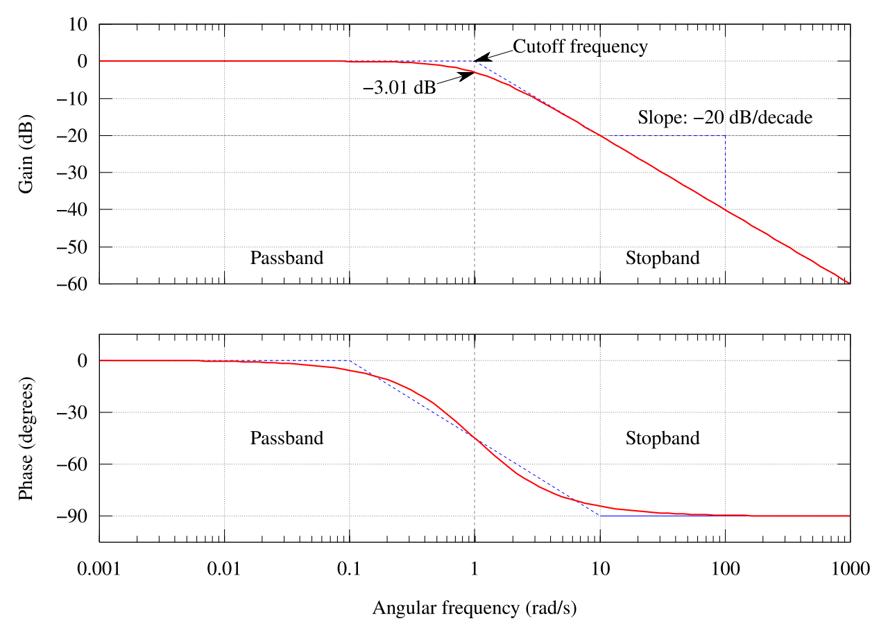
English: The Bode plot of a Butterworth filter with logarithmic axes and various labels. Cutoff frequency is normalized to 1 rad/s. Gain is normalized to 0 dB in the passband. Phase is in degrees because that's typical.
The code is kind of kludgy, but makes a good output. Generated in gnuplot with the script below (save as butterworth_bode_plot.plt and then open in gnuplot). Then it was postprocessed with Inkscape. See Wikipedia graph-making tips. Many orders on one plot: Image:Butterworth orders.png
|
||
| 日期 | 2006年4月26日 (上传日期) | ||
| 来源 | 自己的作品 | ||
| 作者 | Alejo2083 | ||
| 其他版本 |
[] .svg:
.png:
|
||
| gnuplot source | click to expand
set terminal svg enhanced size 1250 875 fname "Times" fsize 25
set output "Butterworth_filter_bode_plot.svg"

# Butterworth amplitude response and decibel calculation.  n is the order, which is just 1 in this image.
G(w,n) = 1 / (sqrt(1 + w**(2*n)))
dB(x) = 20 * log10(abs(x))
# Phase is for first order
P(w) = -atan(w)*180/pi


# Gridlines
set grid

# Set x axis to logarithmic scale
set logscale x 10

# No need for a key
set nokey #0.1,-25

# Frequency response's line plotting style
set style line 1 lt 1 lw 2

# Asymptote lines and slope lines are the same "arrow" style
set style line 3 lt 3 lw 1
set style arrow 3 nohead ls 3

# -3 dB arrow style
set style line 4 lt 4 lw 1
set style arrow 4 head filled size screen 0.02,15,45 ls 4

# Separator between passband and stopband line style
set style line 2 lt 2 lw 1
set style arrow 2 nohead ls 2


set multiplot

# Magnitude response
# =============================================
set size 1,0.5
set origin 0,0.5

# Set range of x and y axes
set xrange [0.001:1000]
set yrange [-60:10]

# Create x-axis tic marks once per decade (every multiple of 10)
set xtics 10
#set ytics 10

# No need for two sets of numbers
set format x ""

# Use 10 x-axis minor divisions per major division
set mxtics 10

# Axis labels
set ylabel "Gain (dB)"

# Draw asymptote lines
set arrow 1 from 1,0 to 1000,-60 as 3
set arrow 2 from .001,0 to 1,0 as 3

# -3 dB arrow
set arrow 4 from 2,3 to 1,0 as 4

# "Cutoff frequency" label uses same coordinates as the function
set label 3 "Cutoff frequency" at 2,4 l

# "-3 dB" label
set arrow 5 from 0.5,-6 to 1,-3 as 4
set label 4 "-3.01 dB" at 0.5,-7 r

# Draw a separator between passband and stopband and label them
set arrow 3 from 1,-60 to 1,10 as 2

# Label coordinates are relative to the graph window, not to the function, centered at the 1/4 and 3/4 width points
set label 1 "Passband" at graph 0.25, graph 0.1 c
set label 2 "Stopband" at graph 0.75, graph 0.1 c

# Draw slope lines and label
set arrow 6 from 100,-20 to 12,-20 as 3
set arrow 7 from 100,-20 to 100,-39 as 3
set label 5 "Slope: -20 dB/decade" at 100,-15 c

plot dB(G(x,1)) ls 1  title "1st-order response"


#Phase response
# =============================================
set size 1,0.5
set origin 0,0

# Set range of x and y axes
set yrange [-105:15]

# Create y-axis tic marks every 15 degrees
set ytics 30

# Regular numbers
set format x "% g"

# Axis labels
set ylabel "Phase (degrees)"
set xlabel "Angular frequency (rad/s)"

# Draw asymptote lines
set arrow 1 from 0.1,0 to 10,-90 as 3
set arrow 2 from 0.001,0 to 0.1,0 as 3
set arrow 10 from 10,-90 to 1000,-90 as 3

# -3 dB arrow
unset arrow 4 #from 2,3 to 1,0 as 4

# "Cutoff frequency" label uses same coordinates as the function
unset label 3 #"Cutoff frequency" at 2,4 l

# "-3 dB" label
unset arrow 5 #from 0.5,-6 to 1,-3 as 4
unset label 4 #"-3.01 dB" at 0.5,-7 r

# Draw a separator between passband and stopband and label them
set arrow 3 from 1,-105 to 1,15 as 2

# Label coordinates are relative to the graph window, not to the function, centered at the 1/4 and 3/4 width points
set label 1 "Passband" at graph 0.25, graph 0.5 c
set label 2 "Stopband" at graph 0.75, graph 0.5 c

# Draw slope lines and label
unset arrow 6 #from 100,-20 to 12,-20 as 3
unset arrow 7 #from 100,-20 to 100,-39 as 3
unset label 5 #"Slope: -20 dB/decade" at 100,-18 c

plot P(x) ls 1 title "Phase response"


unset multiplot
|


|
此图片的光栅版本可用。如果效果更好,那么该栅格图片应当替换本图片。
File:Butterworth filter bode plot.svg → File:Butterworth filter bode plot.png
通常,最好使用好的矢量版本(SVG)。 |
 |
许可协议
我,本作品著作权人,特此采用以下许可协议发表本作品:

|
已授权您依据自由软件基金会发行的无固定段落及封面封底文字(Invariant Sections, Front-Cover Texts, and Back-Cover Texts)的GNU自由文件许可协议1.2版或任意后续版本的条款,复制、传播和/或修改本文件。该协议的副本请见“GNU Free Documentation License”。 |
| 本文件采用知识共享署名-相同方式共享 3.0 未本地化版本许可协议授权。 | ||
| ||
| 本许可协议标签作为GFDL许可协议更新的组成部分被添加至本文件。 |
- 您可以自由地:
- 共享 – 复制、发行并传播本作品
- 修改 – 改编作品
- 惟须遵守下列条件:
- 署名 – 您必须对作品进行署名,提供授权条款的链接,并说明是否对原始内容进行了更改。您可以用任何合理的方式来署名,但不得以任何方式表明许可人认可您或您的使用。
- 相同方式共享 – 如果您再混合、转换或者基于本作品进行创作,您必须以与原先许可协议相同或相兼容的许可协议分发您贡献的作品。
您可以选择您需要的许可协议。
文件历史
点击某个日期/时间查看对应时刻的文件。
| 日期/时间 | 缩略图 | 大小 | 用户 | 备注 | |
|---|---|---|---|---|---|
| 当前 | 2023年10月12日 (四) 03:39 | | 1,250 × 875(31 KB) | wikimediacommons>Mikhail Ryazanov | +ru translation |
文件用途
以下页面使用本文件: